Trying Kolmogorov-Arnold Networks in Practice

There's been a fair bit of buzz about Kolmogorov-Arnold networks online lately. Some research papers were posted around claiming that they offer better accuracy or faster training compared to traditional neural networks/MLPs for the same parameter count.

I was compelled by these claims and decided to test them out myself. Here are my main findings if you're not interested in reading through the details:

That being said, KANs can usually come close to or match the performance of regular neural networks at the same parameter count. However, they are much more complicated to implement than neural networks and require a lot of tricks and hacky-feeling techniques to make them work.

I do believe that there are specialized use cases where they could be objectively better than NNs and be worth pursuing, but in my opinion the brutal simplicity of NNs make them a much stronger default choice.

KAN Background

Here's a diagram representing a minimal KAN:

And here's a neural network/multi-layer perceptron with the same number of layers and nodes:

One big difference to note is that there are far fewer connections between nodes in KANs compared to neural networks/MLPs. KANs move the majority of the learnable parameters into the nodes/activation functions themselves.

B-Splines

The usual choice of learnable activation function used by KANs is the B-Spline.

B-splines are fancy little mathematical gizmos which are composed of multiple piecewise n-degree polynomials strung together in such a way that they're continuous at every point. Here's an example:

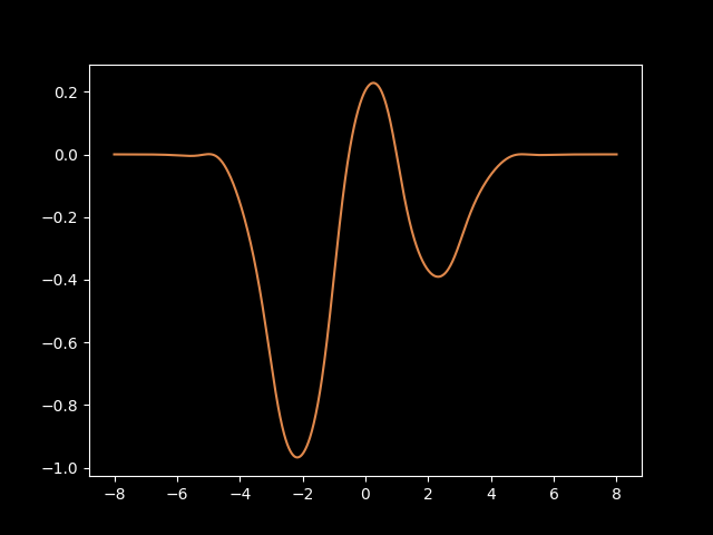
There's a lot of things you can customize with B-splines. You can pick the degree of polynomial used to represent the different grid segments, you can pick the number of knots which determines how many polynomials are strung together, and you can specify the domain/range of the spline however you want.

Another nice thing about B-splines is that they are entirely differentiable. That means that the autograd implementations in machine learning frameworks like Torch, Jax, and Tinygrad can optimize the coefficients used to define the splines directly. This is how the "learning" in machine learning happens, so definitely something that's needed for an activation function to be usable in a KAN.

KANs in Practice

After reading up enough on KANs to feel like I understood what was going on, I decided to try implementing them myself from scratch and try them out on some toy problems. I decided to build it in Tinygrad, a minimal ML framework I've had success working with in the past. What I ended up with is here.

The basic KAN architecture wasn't too complicated, and the only really tricky part was the B-spline implementation. For that, I just ported the implementation that the authors of the original KAN research paper created for their PyKAN library.

Simple 1D Test Function

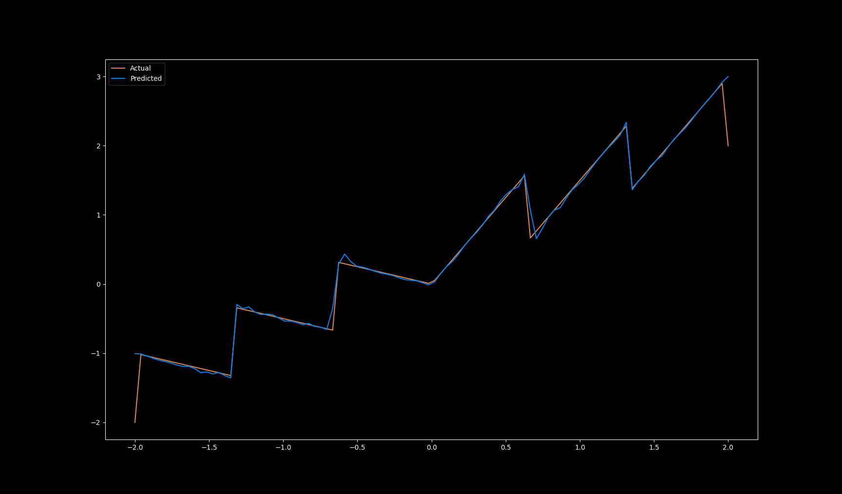
After a bit of effort and some debugging, I had a working KAN implementation. To test it out, I set up a small KAN with 2 layers and trained it to fit some relatively simple 1D functions and it did a pretty good job:

To understand what kind of splines it was learning to accomplish this, I plotted the output of each spline in the network across the full input range of the model:

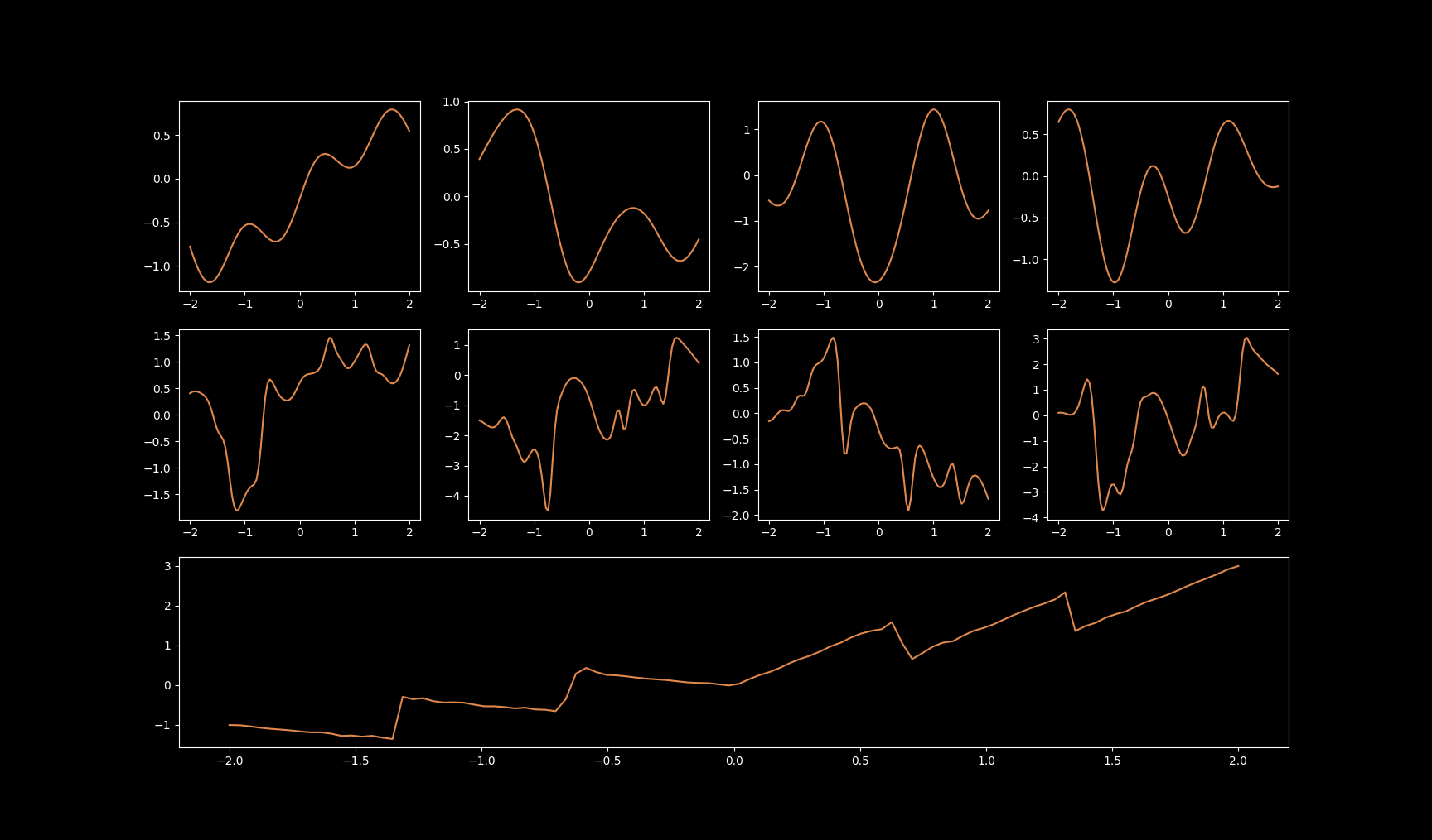
Pretty solid results! The first layer's outputs are pretty simple and represent a single spline each. Then the second layer creates more complicated representations that are stitched together from the outputs of the previous layer, and the final layer has a single spline which combines it all together and returns the model's output.

Scaling Up

Inspired by this early success, I decided to try turning up the complexity. I set up a training pipeline to parameterize images - learning a function like (normalizedXCoord, normalizedYCoord) -> pixelLuminance.

I used a version of positional encoding to expand the coordinates from single scalars into small vectors to make it easier for the networks to learn high-frequency features.

The models would fail to converge or perform badly. I tried changing a bunch of things like layer count, knot count and spline order on the splines, learning rate, you name it. Some things helped, but it was largely a pretty poor showing.

At some point, I figured I'd take a look at PyKAN's source code to see if I was missing something in my implementation compared to what they were doing. I'd had good luck with PyKAN when testing it out in a Python notebook when I was first investigating KANs.

As it turns out, there was a whole lot more going on there than I expected.

PyKAN's Tricks and Extras

PyKAN's source code is actually pretty small and easy enough to parse through.

Here are the ones I noticed:

Bias

PyKAn includes a learnable bias vector which is added to the output of each layer before passing it to the next. This is the same thing that traditional neural networks have.

They include this note in the docs:

biases are added on nodes (in principle, biases can be absorbed into activation functions. However, we still have them for better optimization)

I added them to my own KAN implementation and sure enough, I did see an improvement in learning ability.

Spline Weights

I also noticed that PyKAN was using a learnable weight vector of size (in_count * out_count,) and multiplying the output of the splines by this before summing.

This is a pretty big vector, and it scales multiplicatively with the layer width. It's actually as big as the entire weight vector for a dense layer of a traditional neural network.

That being said, it seems to be worth it. When I added it to my KAN implementation and trimmed down the layer sizes to keep the param count the same, the training performance was about the same or slightly better.

Base Functions

In addition to the B-Splines, the PyKAN implementation also included something they call "base functions", also referred to as "residual functions".

Not to be confused with the basis functions which are used internally in the B-Spline implementation, these add a different path for data to get through the layer that bypasses the splines entirely. The function used defaults to torch.nn.SiLU() which is a close relative of the ReLU activation function.

So the input vector of the layer gets passed through this base function element-wise, multiplied by yet another set of learnable weights of shape (in_count * out_count), and then added to the outputs of the splines.

So there's really a lot going on now, and we're quite far away from the simple architecture from the diagram I included earlier. The KAN layer is something like this now:

y = (splines(x) * spline_weights + base_fn(x) * base_weights).sum(axis=-1) + bias

Grid Updates + Extensions

There's also a lot of code included for things they call grid extensions and grid updates. I believe that these are for dynamically adjusting the domain of individual splines and/or the number of knots in a spline live during training.

There was an example on the PyKAN Github showing how they'd refine the splines to add more and more knots and provide higher and higher resolution. They'd pick new coefficients to approximate the old spline as closely as possible so it could be done during training.

I didn't mess with any of these and definitely didn't attempt porting them over to my Tinygrad implementation.

LBFGS Optimizer

Finally, I noticed that they were using an optimizer called LBFGS to tune their parameters instead of the SGD or Adam that are usually seen when training neural networks.

I looked into it a little bit and found a Wikipedia page. Here's the first sentence from that:

Limited-memory BFGS (L-BFGS or LM-BFGS) is an optimization algorithm in the family of quasi-Newton methods that approximates the Broyden–Fletcher–Goldfarb–Shanno algorithm (BFGS)

I didn't attempt to dig into that further, but I figure that they got better results with that compared to more commonly used optimizers.

Results

I integrated a few of these techniques - specifically the base function + base weights, spline weights, and bias vector - into my Tinygrad KAN implementation. Since these add a huge amount of parameters to the model, I had to significantly reduce the layer sizes and counts that I was testing with in order to keep the same param count.

Despite that, they did seem to help - some more than others - but they also slowed training down a ton.

B-Spline Alternatives

I come from a software development background, and seeing all of these "extras" and special techniques mixed into the KAN implementation felt like a sort of code smell to me.

I wanted to see if I could implement a much more minimal version of a KAN which retained its cool property of having a learnable activation function in a simpler way.

I experimented with some different options for a while and eventually landed on an activation function like this:

y = tanh(a * x.pow(2) + b * x)

Where both a and b are learnable.

I got pretty decent results, coming relatively close to the Spline-based KANs on the image parameterization use case and training like 10x faster as well. I mixed in the learnable bias and played around with some other variations, but the improvements were small or negative.

Eventually, it got to the point where I was just dancing around the same final loss value +-20% or so and I stopped my search.

Conclusion

I spent a few more days trying different variations on this theme: mixing KAN layers and NN layers, tweaking model width vs. depth, tuning various other hyperparameters like learning rate and batch size. Despite my efforts, the results were the same:

I was able to train a model to a loss of 0.0006 after 20k epochs with a neural network using boring tanh activations, and the best I could do with the most successful training run with a KAN was about 0.0011.

I'll admit that there's a decent chance I missed something in my KAN implementation, failed to find the architecture of hyperparameters that would work best for me, or picked an unlucky thing to test with that just doesn't work well for KANs.

But the fact that neural networks worked so well with so little effort was pretty compelling and made me uninterested in spending more time trying to get KANs to outperform them for now. In any case, it wasn't anything close to the "50% less params for the same performance" that I'd heard claims of.

One final note is that I really don't want this to come off as me trashing on KANs and saying that they're useless. Some of the demos on the PyKAN Github and docs revolve around more niche or use cases like learning functions to "machine precision" with 64-bit floats - which they do successfully. Neural networks can't do easily if at all.

I think work investigating alternatives or improvements to neural networks is very worthwhile, and might be the kind of thing that gives us the next transformer-level leap in AI capability.