Reverse Engineering a Neural Network's Clever Solution to Binary Addition

There's a ton of attention lately on massive neural networks with billions of parameters, and rightly so. By combining huge parameter counts with powerful architectures like transformers and diffusion, neural networks are capable of accomplishing astounding feats.

However, even small networks can be surprisingly effective - especially when they're specifically designed for a specialized use-case. As part of some previous work I did, I was training small (<1000 parameter) networks to generate sequence-to-sequence mappings and perform other simple logic tasks. I wanted the models to be as small and simple as possible with the goal of building little interactive visualizations of their internal states.

After finding good success on very simple problems, I tried training neural networks to perform binary addition. The networks would receive the bits for two 8-bit unsigned integers as input (converted the bits to floats as -1 for binary 0 and +1 for binary 1) and would be expected to produce properly-added output, including handling wrapping of overflows.

Training example in binary:

  01001011 + 11010110 -> 00100001

As input/output vectors for NN training:

  input:  [-1, 1, -1, -1, 1, -1, 1, 1, 1, 1, -1, 1, -1, 1, 1, -1]
  output: [-1, -1, 1, -1, -1, -1, -1, 1]

What I hoped/imagined the network would learn internally is something akin to a binary adder circuit:

I expected that it would identify the relationships between different bits in the input and output, route them around as needed, and use the neurons as logic gates - which I'd seen happen in the past for other problems I tested.

Training the Network

To start out, I created a network with a pretty generous architecture that had 5 layers and several thousand parameters. However, I wasn't sure even that was enough. The logic circuit diagram above for the binary adder only handles a single bit; adding 8 bits to 8 bits would require a much larger number of gates, and the network would have to model all of them.

Additionally, I wasn't sure how the network would handle long chains of carries. When adding 11111111 + 00000001, for example, it wraps and produces an output of 00000000. In order for that to happen, the carry from the least-significant bit needs to propagate all the way through the adder to the most-significant bit. I thought that there was a good chance the network would need at least 8 layers in order to facilitate this kind of behavior.

Even though I wasn't sure if it was going to be able to learn anything at all, I started off training the model.

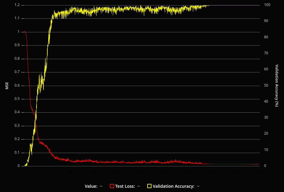
I created training data by generating random 8-bit unsigned integers and adding them together with wrapping. In addition to the loss computed during training of the network, I also added code to validate the network's accuracy on all 32,385 possible input combinations periodically during training to get a feel for how well it was doing overall.

After some tuning of hyperparameters like learning rate and batch size, I was surprised to see that the model was learning extremely well! I was able to get it to the point where it was converging to perfect or nearly perfect solutions almost every training run.

I wanted to know what the network was doing internally to generate its solutions. The networks I was training were pretty severely overparameterized for the task at hand; it was very difficult to get a grasp of what they were doing through the tens of thousands of weights and biases. So, I started trimming the network down - removing layers and reducing the number of neurons in each layer.

To my continued surprise, it kept working! At some point perfect solutions became less common as networks become dependent on the luck of their starting parameters, but I was able to get it to learn perfect solutions with as few as 3 layers with neuron counts of 12, 10, and 8 respectively:

Layer (type)           Input Shape    Output shape  Param #
===========================================================
input1 (InputLayer)    [[null,16]]    [null,16]     0
___________________________________________________________
dense_Dense1 (Dense)   [[null,16]]    [null,12]     204
___________________________________________________________
dense_Dense2 (Dense)   [[null,12]]    [null,10]     130
___________________________________________________________
dense_Dense3 (Dense)   [[null,10]]    [null,8]      88
===========================================================

That's just 422 total parameters! I didn't expect that the network would be able to learn a complicated function like binary addition with that few.

It seemed too good to be true, to be honest, and I wanted to make sure I wasn't making some mistake with the way I was training the network or validating its outputs. A review of my example generation code and training pipeline didn't reveal anything that looked off, so the next step was to actually take a look at the parameters after a successful training run.

Unique Activation Functions

One important thing to note at this point is the activation functions used for the different layers in the model. Part of my previous work in this area consisted of designing and implementing a new activation function for use in neural networks with the goal of doing binary logic as efficiently as possible. Among other things, it is capable of modeling any 2-input boolean function in a single neuron - meaning that it solves the XOR problem.

You can read about it in more detail in my other post, but here's what it looks like:

It looks a bit like a single period of a flattened sine wave, and it has a couple controllable parameters to configure how flat it is and how it handles out-of-range inputs.

For the models I was training for binary addition, all of them used this activation function (which I named Ameo) in the first layer and used tanh for all the other layers.

Dissecting the Model

Although the number of parameters was now pretty manageable, I couldn't discern what was going on just by looking at them. However, I did notice that there were lots of parameters that were very close to "round" values like 0, 1, 0.5, -0.25, etc.

Since lots of the logic gates I'd modeled previously were produced with parameters such as those, I figured that might be a good thing to focus on to find the signal in the noise.

I added some rounding and clamping that was applied to all network parameters closer than some threshold to those round values. I applied it periodically throughout training, giving the optimizer some time to adjust to the changes in between. After repeating several times and waiting for the network to converge to a perfect solution again, some clear patterns started to emerge:

layer 0 weights:
[[0         , 0         , 0.1942478 , 0.3666477, -0.0273195, 1         , 0.4076445 , 0.25     , 0.125    , -0.0775111, 0         , 0.0610434],
 [0         , 0         , 0.3904364 , 0.7304437, -0.0552268, -0.0209046, 0.8210054 , 0.5      , 0.25     , -0.1582894, -0.0270081, 0.125    ],
 [0         , 0         , 0.7264696 , 1.4563066, -0.1063093, -0.2293   , 1.6488117 , 1        , 0.4655252, -0.3091895, -0.051915 , 0.25     ],
 [0.0195805 , -0.1917275, 0.0501585 , 0.0484147, -0.25     , 0.1403822 , -0.0459261, 1.0557909, -1       , -0.5      , -0.125    , 0.5      ],
 [-0.1013674, -0.125    , 0         , 0        , -0.4704586, 0         , 0         , 0        , 0        , -1        , -0.25     , -1       ],
 [-0.25     , -0.25     , 0         , 0        , -1        , 0         , 0         , 0        , 0        , 0.2798074 , -0.5      , 0        ],
 [-0.5      , -0.5226266, 0         , 0        , 0         , 0         , 0         , 0        , 0        , 0.5       , -1        , 0        ],
 [1         , -0.9827325, 0         , 0        , 0         , 0         , 0         , 0        , 0        , -1        , 0         , 0        ],
 [0         , 0         , 0.1848682 , 0.3591821, -0.026541 , -1.0401837, 0.4050815 , 0.25     , 0.125    , -0.0777296, 0         , 0.0616584],
 [0         , 0         , 0.3899804 , 0.7313382, -0.0548765, -0.021433 , 0.8209481 , 0.5      , 0.25     , -0.156925 , -0.0267142, 0.125    ],
 [0         , 0         , 0.7257989 , 1.4584024, -0.1054092, -0.2270812, 1.6465081 , 1        , 0.4654536, -0.3099159, -0.0511372, 0.25     ],
 [-0.125    , 0.069297  , -0.0477796, 0.0764982, -0.2324274, -0.1522287, -0.0539475, -1       , 1        , -0.5      , -0.125    , 0.5      ],
 [-0.1006763, -0.125    , 0         , 0        , -0.4704363, 0         , 0         , 0        , 0        , -1        , -0.25     , 1        ],
 [-0.25     , -0.25     , 0         , 0        , -1        , 0         , 0         , 0        , 0        , 0.2754751 , -0.5      , 0        ],
 [-0.5      , -0.520548 , 0         , 0        , 0         , 0         , 0         , 0        , 0        , 0.5       , 1         , 0        ],
 [-1        , -1        , 0         , 0        , 0         , 0         , 0         , 0        , 0        , -1        , 0         , 0        ]]

layer 0 biases:
[0          , 0         , -0.1824367,-0.3596431, 0.0269886 , 1.0454538 , -0.4033574, -0.25    , -0.125   , 0.0803178 , 0         , -0.0613749]

Above are the final weights generated for the first layer of the network after the clamping and rounding. Each column represents the parameters for a single neuron, meaning that the first 8 weights from top to bottom are applied to bits from the first input number and the next 8 are applied to bits from the second one.

All of these neurons have ended up in a very similar state. There is a pattern of doubling the weights as they move down the line and matching up weights between corresponding bits of both inputs. The bias was selected to match the lowest weight in magnitude. Different neurons had different bases for the multipliers and different offsets for starting digit.

The Network's Clever Solution

After puzzling over that for a while, I eventually started to understand how its solution worked.

Digital to analog converters (DACs) are electronic circuits that take digital signals split into multiple input bits and convert them into a single analog output signal.

DACs are used in applications like audio playback where a sound files are represented by numbers stored in memory. DACs take those binary values and convert them to an analog signal which is used to power the speakers, determining their position and vibrating the air to produce sound. For example, the Nintendo Game Boy had a 4-bit DAC for each of its two output audio channels.

Here's an example circuit diagram for a DAC:

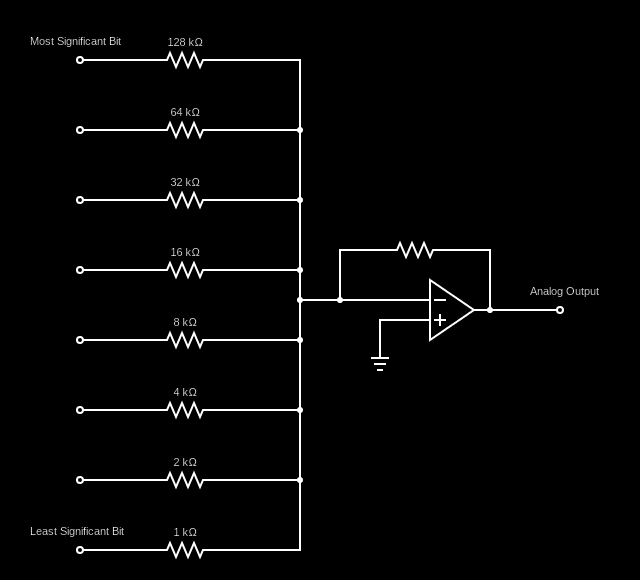
If you look at the resistances of the resistors attached to each of the bits of the binary input, you can see that they double from one input to another from the least significant bit to the most significant. This is extremely similar to what the network learned to do with the weights of the input layer. The main difference is that the weights are duplicated between each of the two 8-bit inputs.

This was only part of the puzzle, though. Once the digital inputs were converted to analog and summed together, they were immediately passed through the neuron's activation function. To help track down what happened next, I plotted the post-activation outputs of a few of the neurons in the first layer as the inputs increased:

The neurons seemed to be generating sine wave-like outputs that changed smoothly as the sum of the binary inputs increased. Different neurons had different periods; the ones pictured above have periods of 8, 4, and 32 respectively. Other neurons had different periods or were offset by certain distances.

There's something very remarkable about this pattern: they map directly to the periods at which different binary digits switch between 0 and 1 when counting in binary. The least significant digit switches between 0 and 1 with a period of 1, the second with a period of 2, and so on to 4, 8, 16, 32, etc. This means that for at least some of the output bits, the network had learned to compute everything it needed in a single neuron.

Looking at the weights of neurons in the two later layers confirms this to be the case. The later layers are mostly concerned with routing around the outputs from the first layer and combining them. One additional benefit that those layers provide is "saturating" the signals and making them more square wave-like - pushing them closer to the target values of -1 and 1 for all values. This is the exact same property which is used in digital signal processing for audio synthesis where tanh is used to add distortion to sound for things like guitar pedals.

While playing around with this setup, I tried re-training the network with the activation function for the first layer replaced with sin(x) and it ends up working pretty much the same way. Interestingly, the weights learned in that case are fractions of π rather than 1.

For other output digits, the network learned to do some over clever things to generate the output signals it needed. For example, it combined outputs from the first layer in such a way that it was able to produce a shifted version of the signal not present in any of the first-layer neurons by adding signals from other neurons with different periods together. It worked out pretty well, more than accurate enough for the purpose of the network.

The sine-based version of the function learned by the network (blue) ends up being roughly equivalent to the function sin(1/2x + pi) (orange):

I have no idea if this is just another random mathematical coincidence or part of some infinite series or something, but it's very neat regardless.

Summary

So, in all, the network was accomplishing binary addition by:

1. Converting the binary inputs into "analog" using a version of a digital to analog converter implemented using the weights of the input layer
2. Mapping that internal analog signal into periodic sine wave-like signals using the Ameo activation function (even though that activation function isn't periodic)
3. Saturating the sine wave-like signal to make it more like a square wave so outputs are as close as possible to the expected values of -1 and 1 for all outputs

As I mentioned, before, I had imagined the network learning some fancy combination of logic gates to perform the whole addition process digitally, similarly to how a binary adder operates. This trick is yet another example of neural networks finding unexpected ways to solve problems.

Epilogue

One thought that occurred to me after this investigation was the premise that the immense bleeding-edge models of today with billions of parameters might be able to be built using orders of magnitude fewer network resources by using more efficient or custom-designed architectures.

It's an exciting prospect to be sure, but my excitement is somewhat dulled because I was immediately reminded of The Bitter Lesson. If you've not read it, you should read it now (it's very short); it really impacted the way I look at computing and programming.

Even if this particular solution was just a fluke of my network architecture or the system being modeled, it made me even more impressed by the power and versatility of gradient descent and similar optimization algorithms. The fact that these very particular patterns can be brought into existence so consistently from pure randomness is really amazing to me.

I plan to continue my work with small neural networks and eventually create those visualizations I was talking about. If you're interested, you can subscribe to my blog via RSS at the top of the page, follow me on Twitter @ameobea10, or Mastodon @ameo@mastodon.ameo.dev.